Spatial expansion

Load data

my_colors <- c("#66b803", "#E5AA9B", "#FABD3E", "#2B8CBE", "#DE77AE", "#9970AB", "gray", "#D5E4A2", "#71D0F5", "#B1746F", "#ADE2D0", "#20DE8BFF", "#CCDE8BFF", "#FFDE8BFF", "#FFA88BFF", "#FF6A8BFF")
load("vignette_data/HCC_1L_obj.rda")
load("vignette_data/HCC_1L_spot_celltype.rda")

The “HCC_1L_obj” data is a Seurat object that has been normalized using SCTransform . This data is mentioned in the section on "Data and Materials Availability "in our paper .

SpaTopic

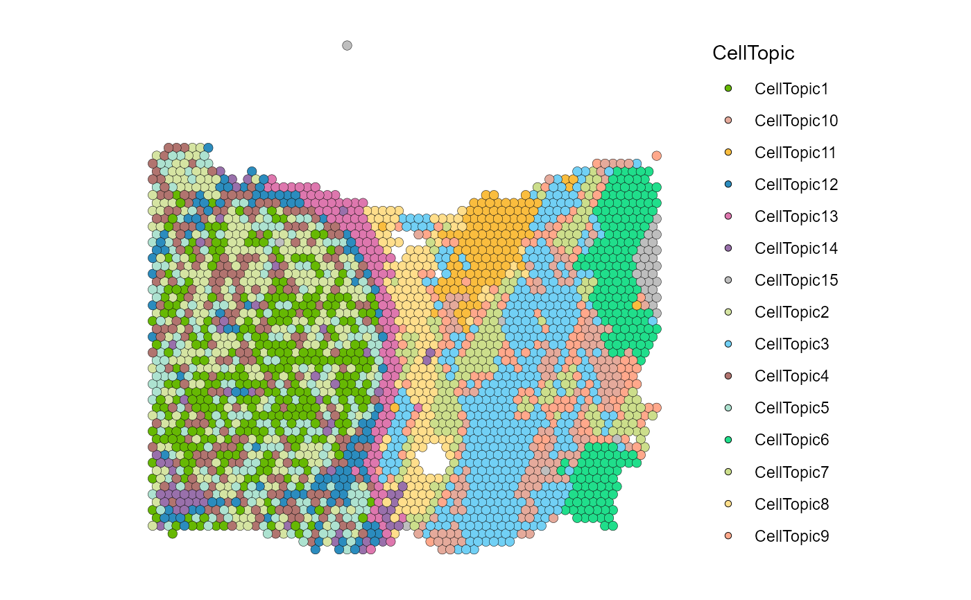
We first use SpaTopic to get the CellTopic of the spatial domain.

HCC_1L_obj <- RunPCA(HCC_1L_obj, assay = "SCT", verbose = FALSE)
HCC_1L_obj <- FindNeighbors(HCC_1L_obj, reduction = "pca", dims = 1:30)
HCC_1L_obj <- FindClusters(HCC_1L_obj, resolution = 1.5)
HCC_1L_obj <- RunUMAP(HCC_1L_obj, reduction = "pca", dims = 1:30)
HCC_1L_spot_clusters <- HCC_1L_obj@meta.data["seurat_clusters"]
result_list <- CellTopic(
  HCC_1L_spot_celltype,
  HCC_1L_spot_clusters,
  cluster = "seurat_clusters",
  num_topics = 10,
  percent = 0.7
)
HCC_1L_obj <- AddMetaData(HCC_1L_obj, result_list[["CellTopic"]])
SpatialDimPlot(HCC_1L_obj, group.by = "CellTopic", image.alpha = 0, pt.size.factor = 2.2) + scale_fill_manual(values = my_colors)

Modularity Optimizer version 1.3.0 by Ludo Waltman and Nees Jan van Eck

Number of nodes: 2791
Number of edges: 103726

Running Louvain algorithm...
Maximum modularity in 10 random starts: 0.7420
Number of communities: 16
Elapsed time: 0 seconds

Spatial_expansion then divides buffers and angles for the specified spatial domain. It is worth noting that this method is not only applicable to SpaTopic, but also to arbitrary spatial partitions with certain continuity.

We divide the buffers and angles of the spatial domain of the tumor boundary by specifying CellTopic column in Seurat@meta.data, and CellTopic8 in it.

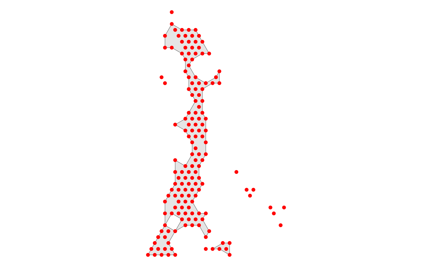
HCC_1L_obj <- Spatial_expansion(HCC_1L_obj,
    CellTopic = c("CellTopic8"),
    meta.col = "CellTopic",
    type = "Hexagon",
    edge.plot = TRUE
)

Use the low resolution image
The type of data is Hexagon 
The alpha value of alpha-shape method is 232 
The distance of expansion is 200 
The expansion of the data is added to the Seurat@meta.data and the message is added to Seurat@misc

When set edge.plot = TRUE, the function draw a reference plot representing the specified spatial domain divide. We can obtain a more appropriate spatial domain divide by modifying the alpha parameter of alpha-shape calculation.

We can check the relevant parameter settings in Seurat@misc as a reference for our adjustments

HCC_1L_obj@misc$expansion$CellTopic8[1:5]

$distance
[1] 200

$alpha
[1] 232

$type
[1] "Hexagon"

$image
[1] "lowres"

$image.factor
[1] 0.02920561

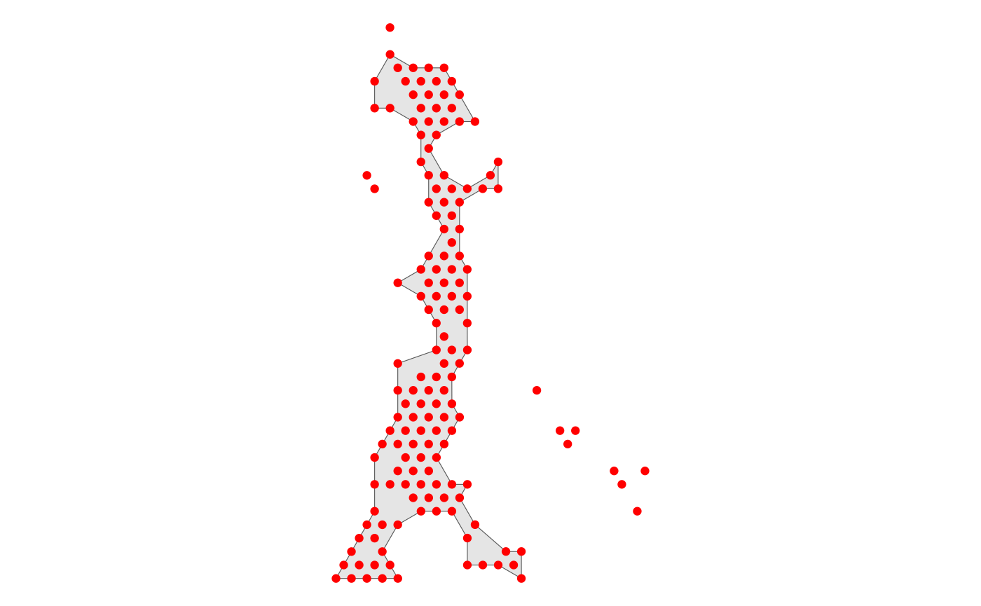
Here we get a more appropriate spatial domain divide by setting alpha = 280.

HCC_1L_obj <- Spatial_expansion(HCC_1L_obj,
    CellTopic = c("CellTopic8"),
    meta.col = "CellTopic",
    alpha = 280,
    type = "Hexagon",
    edge.plot = TRUE
)

Use the low resolution image
The type of data is Hexagon 
The alpha value of alpha-shape method is 280 
The distance of expansion is 200 
The expansion of the data is added to the Seurat@meta.data and the message is added to Seurat@misc

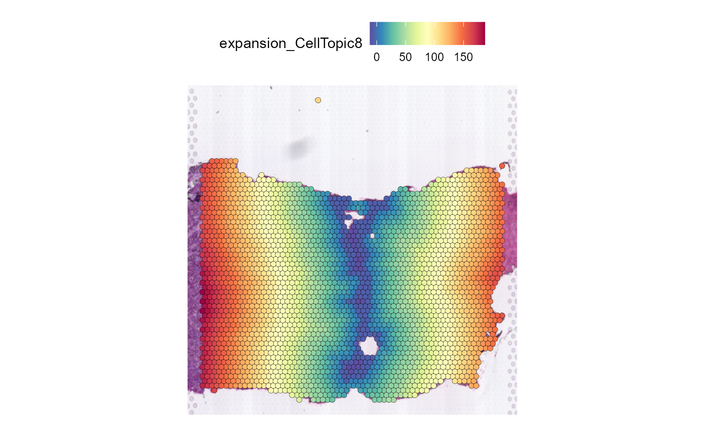
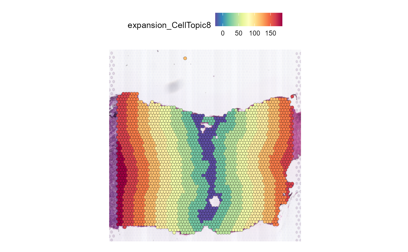
We can use SpatialFeaturePlot in Seurat to show buffer divide of spatial domain.

SpatialFeaturePlot(HCC_1L_obj, features = "expansion_CellTopic8", pt.size.factor = 2.2)

On the other hand, you can increase or decrease the width of the buffers by setting distance .

HCC_1L_obj_1 <- Spatial_expansion(HCC_1L_obj,
    CellTopic = c("CellTopic8"),
    meta.col = "CellTopic",
    distance = 800,
    alpha = 280,
    type = "Hexagon",
    edge.plot = FALSE
)
SpatialFeaturePlot(HCC_1L_obj_1, features = "expansion_CellTopic8", pt.size.factor = 2.2)

Use the low resolution image
The type of data is Hexagon 
The alpha value of alpha-shape method is 280 
The distance of expansion is 800 
The expansion of the data is added to the Seurat@meta.data and the message is added to Seurat@misc

Angle

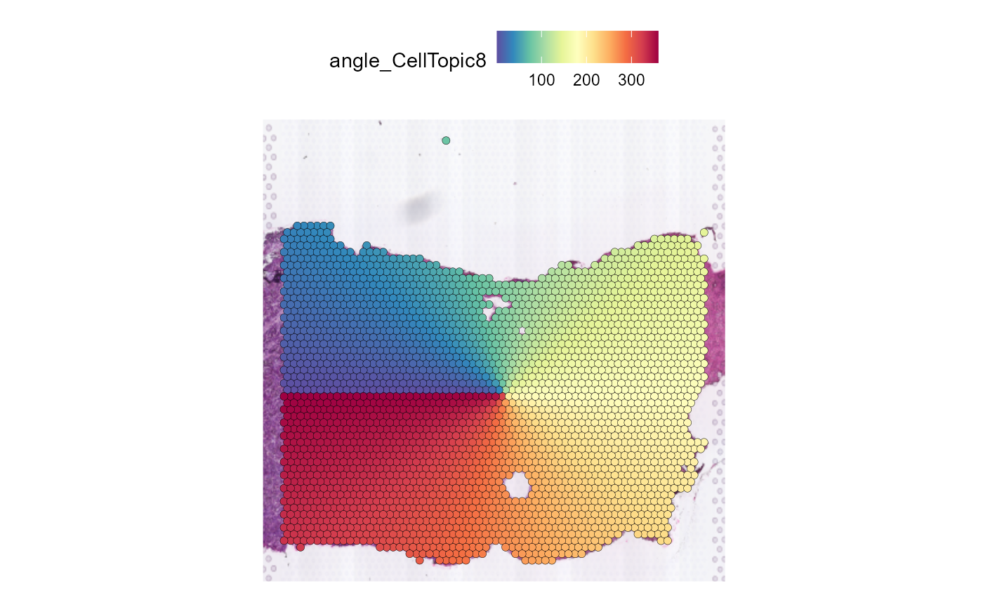
Spatial_expansion creates not only buffer information in Seurat@meta.data, but also angle information.

We regard the geometric center of a spatial domain as the center, and the left side of the spatial domain is the starting point and the ending point of the circle.

SpatialFeaturePlot(HCC_1L_obj, features = "angle_CellTopic8", pt.size.factor = 2.2)

Gene plot

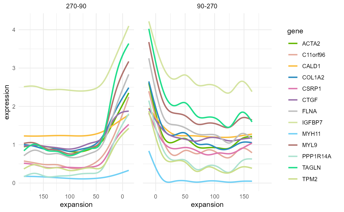
After dividing the spatial domain we can use Expansion_gene_plot to show gene expression changes in buffers in different angles.

Here we set angle = 90, parts = 2 to get gene expression on both sides of the tumor boundary.

Expansion_gene_plot(HCC_1L_obj,
    CellTopic = c("CellTopic8"),
    gene = c("ACTA2", "C11orf96", "CALD1", "COL1A2", "CSRP1", "CTGF", "FLNA", "IGFBP7", "MYH11", "MYL9", "PPP1R14A", "TAGLN", "TPM2"),
    meta.col = "CellTopic", angle = 90, parts = 2, plot = TRUE, cols = my_colors
)

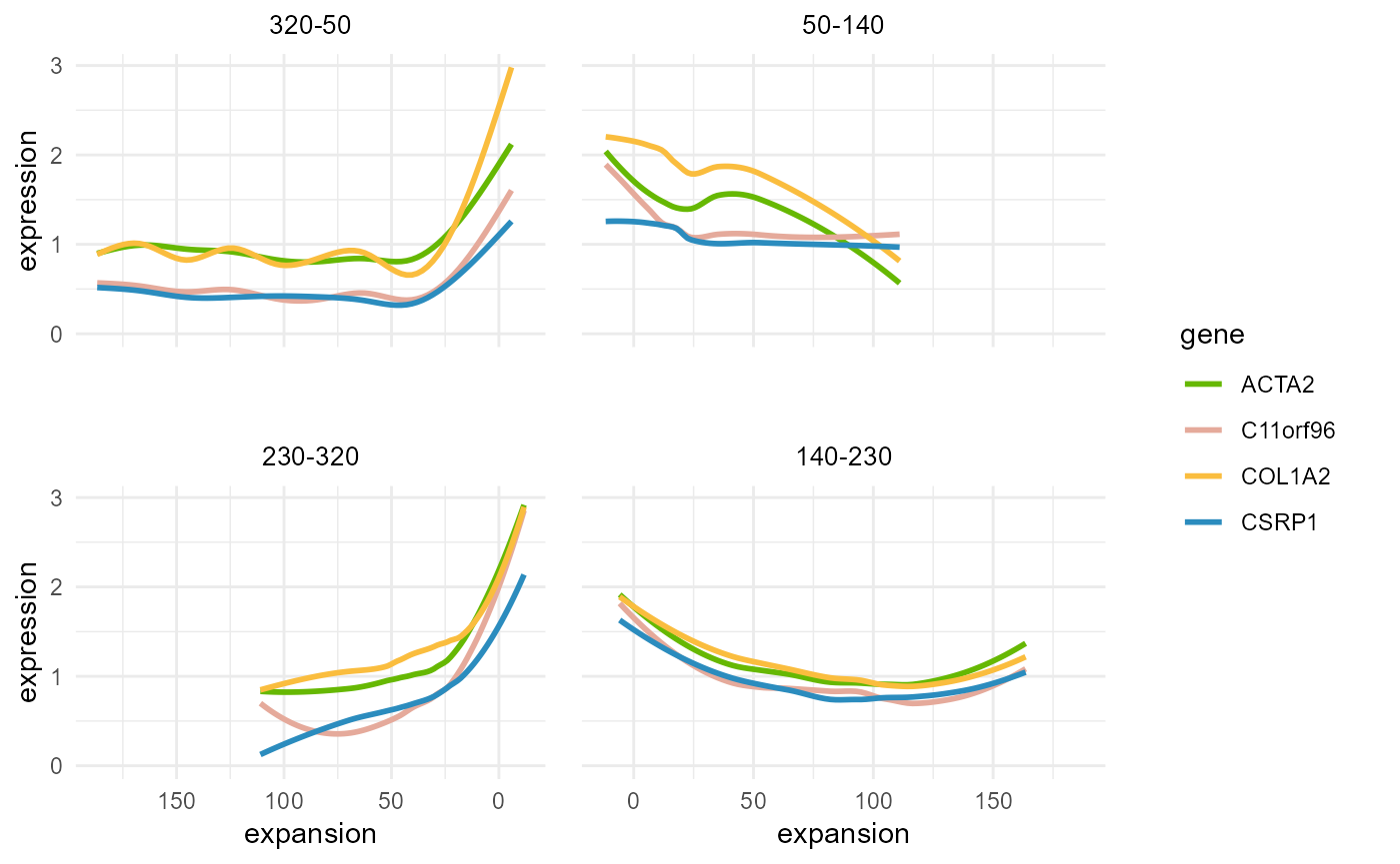
This method was consistent across different angles, as shown when dividing the spatial domain into four sections starting at 50 degrees.

Expansion_gene_plot(HCC_1L_obj,
    CellTopic = c("CellTopic8"),
    gene = c("ACTA2", "C11orf96", "COL1A2", "CSRP1"),
    meta.col = "CellTopic", angle = 50, parts = 4, plot = TRUE, cols = my_colors
)

If you need to plot data for further analysis or re-plotting, you can set plot = FALSE to obtain the expression of genes in buffers at different angles.