Gene regulatory network construction
2023-07-22
Source:vignettes/regulatory_network.Rmd
regulatory_network.RmdGene regulatory networks (GRNs), consisting of the interaction between transcription factors (TFs) and their target genes, orchestrate cell-specific gene expression patterns and in turn determine the function of the cell. To construct cell-type specific GRNs using single-cell data, we have incorporated a widely used single-cell GRN analysis tool SCENIC (Aibar et al., 2017) and a plant specific GRN inference tool MINI-EX (Ferrari et al., 2022) into the scPlant pipeline.
Construct GRNs using SCENIC
We have incorporated the widely used single-cell GRN analysis tool SCENIC (Aibar et al., 2017) into the scPlant pipeline, and prepared required cisTarget databases in order to support SCENIC for data analysis in plants. What’s more, we have provided various visualization tools to display single-cell GRN results in different ways. Three plant species (Arabidopsis thaliana, Oryza sativa, Zea mays) are supported for now, and more plant species will be supported soon.
Download databases and scripts
The required cisTarget databases and scripts to construct gene regulatory network can be downloaded here.
For other species and genome version
Provided cisTarget databases were built based on the following species and genome version:
Arabidopsis thaliana: TAIR10
Oryza sativa: V7.0
Zea mays: Zm-B73-REFERENCE-NAM-5.0
For other species and genome version, users can build their own cisTarget databases by following the protocol create_cisTarget_databases.
Create tbl file for other species
For other species, users can create their own motif2TF.tbl file by creating a data frame with the information of the motifs and their corresponding TFs, which is the most important information in tbl files and can be downloaded from some databases such as JASPAR and PlantTFDB.
Here is the code to create a motif2TF.tbl file:
# Assuming motif2TF is a three-column data frame with the information of motifs and their corresponding TFs like this:
# motif TF source
# MP00120   AT1G01250   PlantTFDB
# MP00100   AT1G01260   PlantTFDB

# Then use the code:
motif2TF <- motif2TF %>% dplyr::transmute(`#motif_id`=motif, motif_name=motif, motif_description=TF,
                                          source_name=source, source_version=1.1, gene_name=TF,
                                          motif_similarity_qvalue=0.000000, similar_motif_id="None",
                                          similar_motif_description="None", orthologous_identity=1.000000,
                                          orthologous_gene_name="None", orthologous_species="None",
                                          description="gene is directly annotated")
write.table(motif2TF, file = "motif2TF.tbl", sep = "\t", row.names = F, quote = F)
We also provide a real scRNA-seq data of Arabidopsis thaliana (Zhang et al., 2019) as example data, download here.
Installation
conda create -n pyscenic_12_1 python=3.8
conda activate pyscenic_12_1
pip install pyscenic==0.12.1
pyscenic -h
Dependent R packages includes optparse,
Seurat, SCopeLoomR, data.table,
pbapply, philentropy, dplyr, if
you have not installed them, start “R” and enter:
install.packages("optparse")
install.packages("Seurat")
devtools::install_github("aertslab/SCopeLoomR")
install.packages("data.table")
install.packages("pbapply")
install.packages("philentropy")
install.packages("dplyr")
Gene regulatory network construction
To read the help information:
USAGE: RunGRN [options]
Run pyscenic and perform post-processing.

-o <output_directory> : Output directory for results.
-f <Seurat_file>        : Seurat object, saved as .rds format.
-s <species>  : Species. Currently At (Arabidopsis thaliana), Os (Oryza sativa), Zm (Zea mays) are supported. For other species, you need to provide your own cisTarget_databases.
-t <threads> : threads. 1 as default.
-d <cisTarget_databases> : directory containing files required to run pyscenic .
Run the script:
output files
Once the program has run successfully, you can find results files in the output directory. You can ignore most of the output files, because only several ones of them are needed for visualization.
# final output files
pyscenicOutput.loom  # loom file containing the original expression matrix and the calculated AUC values
AUCell.txt  # Regulon activity score (RAS) matrix
rasMat.rds # Regulon activity score (RAS) matrix, R object file
rssMat.rds # Regulon Specificity Score (RSS) matrix
tf_target.rds # TF and their targets in each regulon
regulons.gmt  # regulons
regulons.txt # regulons
binary_mtx.txt   # binary regulon activity matrix
# intermediate files
adj.tsv  #  a table of TF-target genes
reg.tsv  # a table of enriched motifs and target genes
exprMat.loom  # loom file of expression matrix
cellmeta.rds  # SeuratObj@meta.data
auc_thresholds.txt  # thresholds to create binary regulon activity matrix
Visualize the GRNs inferred by SCENIC
We provide various visualization tools to display single-cell GRN results in different ways.
Load output files and Seurat object:
rasMat <- readRDS("output/rasMat.rds")
rssMat <- readRDS("output/rssMat.rds")
tf_target <- readRDS("output/tf_target.rds")
SeuratObj <- readRDS("SeuratObj.rds")
Heatmaps showing mean regulon activity and TF expression of each cluster.
ras_exp_hmp(SeuratObj, rasMat, group.by = "cellType", assay = 'SCT')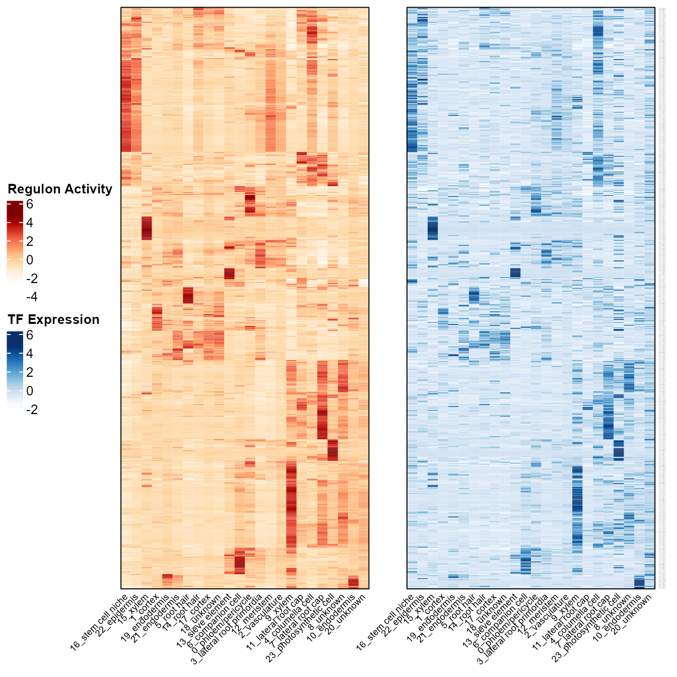
Dimension reduction plot showing regulon activity and TF expression.
ras_exp_scatter(SeuratObj, rasMat, gene = 'AT1G75390', reduction = 'umap')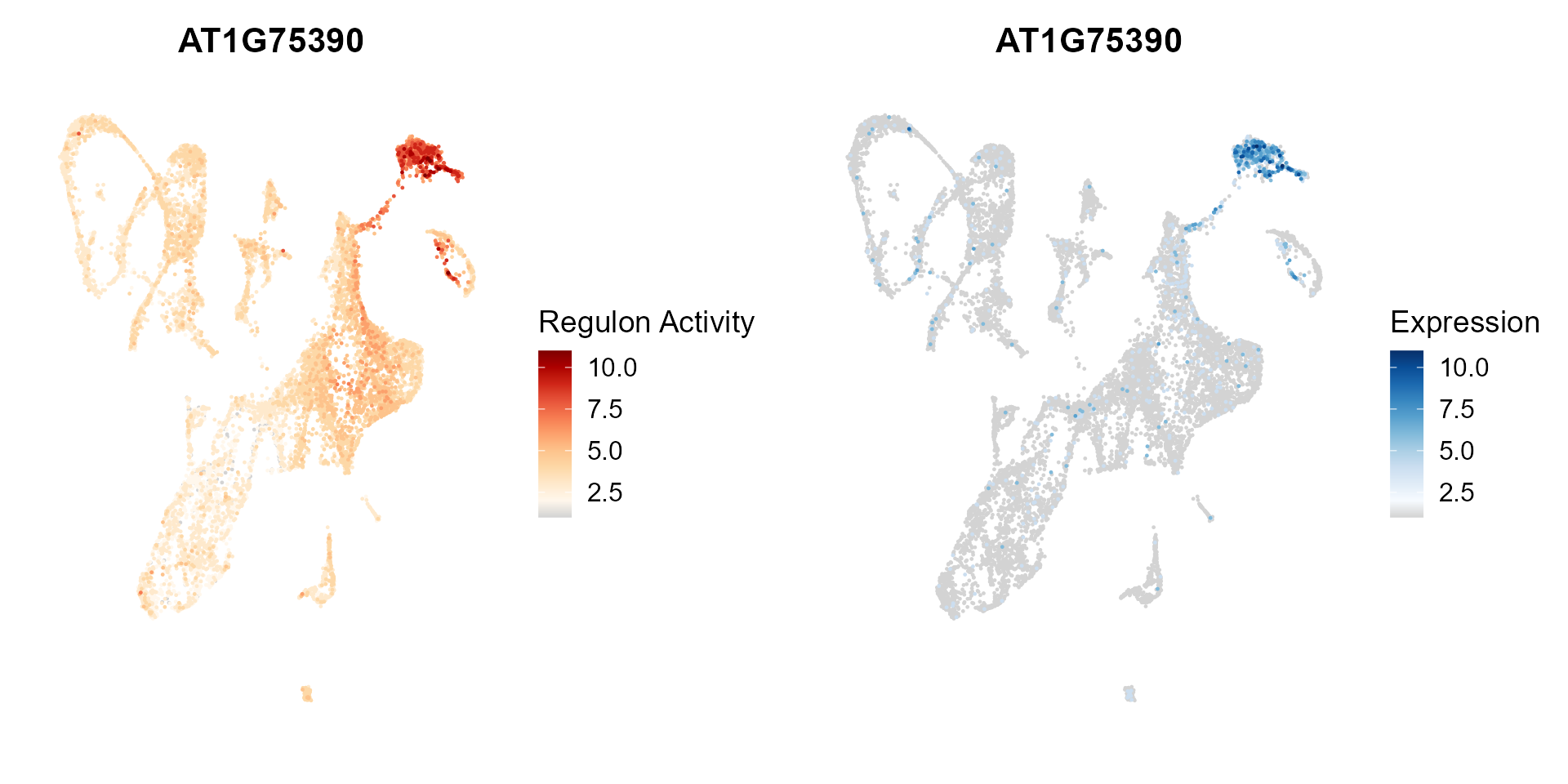
Network diagram showing top regulons of each cluster according to regulon specificity score(RSS).
topRegulons(rssMat, topn = 5)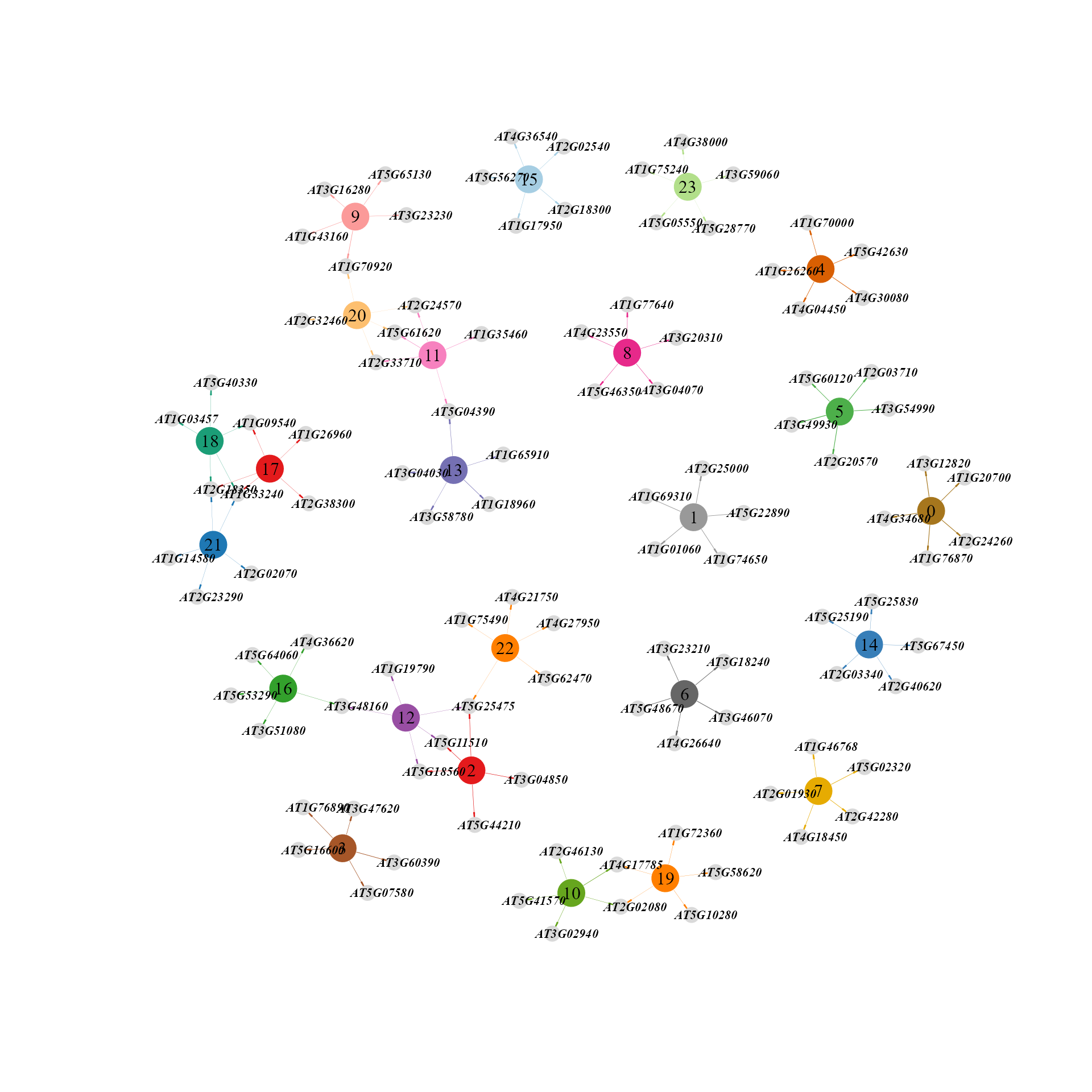
Network diagram showing top targets of each regulon according to importance score.
toptargets(tf_target, topn = 5, regulons = colnames(rasMat)[1:5])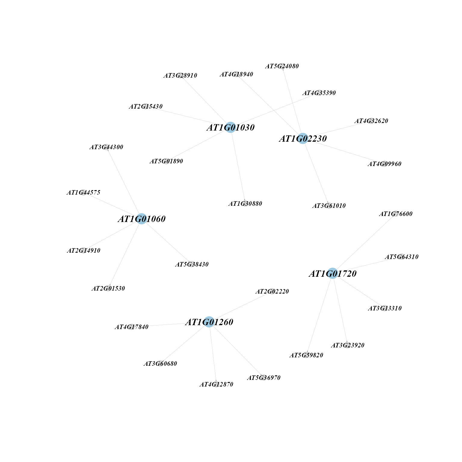
Network diagram showing top targets of top regulons of each cluster.
ToptargetsofTopregulons(rssMat, tf_target, Topregulons = 5, Toptargets = 5)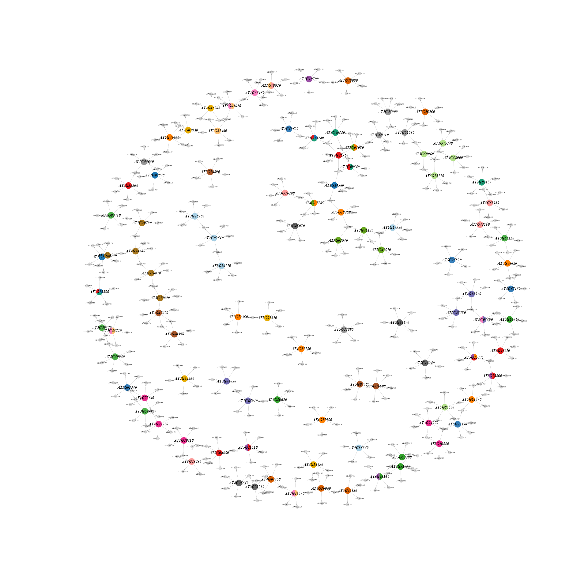
Dot plot showing top regulons of each cluster according to regulon specificity score(RSS).
SpecificityRank(rssMat, cluster = 23, topn = 10)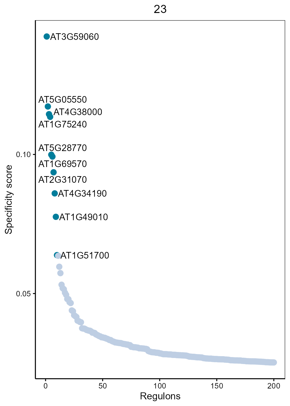
Construct GRNs using MINI-EX
We have incorporated a recently published plant specific GRN inference tool MINI-EX (Ferrari et al., 2022) into the scPlant pipeline. In addition, we have provided various visualization methods to display single-cell GRN results inferred by MINI-EX.
Installation and pre-process
First, we need to download MINI-EX and install the requirements.
To make MINI-EX work properly, Nextflow and Singularity need to be installed. MINI-EX offers a Docker container, but if it doesn’t work, you can create a conda environment and install the requirements manually.
Second, we need to produce the input files for MINI-EX.
We provided a script used to produce the input files for MINI-EX, download here.
We provided a real scRNA-seq data of Arabidopsis thaliana (Zhang et al., 2019) as example data, download here.
unzip scPlantData.zip
Rscript scPlantData/MINIEX_preprocess.R --seuratObj SeuratObj.rds --cluster seurat_clusters --celltype celltype -o INPUTS
Then, modify the miniex.config and change the paths to your own input files generated by the script above. You can modify the parameters according to your particular needs.
Visualize the GRNs inferred by MINI-EX
We have provided various visualization methods to display the GRNs inferred by MINI-EX, which are similar as visualizing the GRNs inferred by SCENIC.
Load the Seurat object and specify the path of output files:
SeuratObj <- readRDS("SeuratObj.rds")
MINIEXouputPath <- "/your_path/regulons_output"
Heatmaps showing cluster enrichment and TF expression of each regulon in each cluster.
enrich_exp_hmp(SeuratObj, MINIEXouputPath)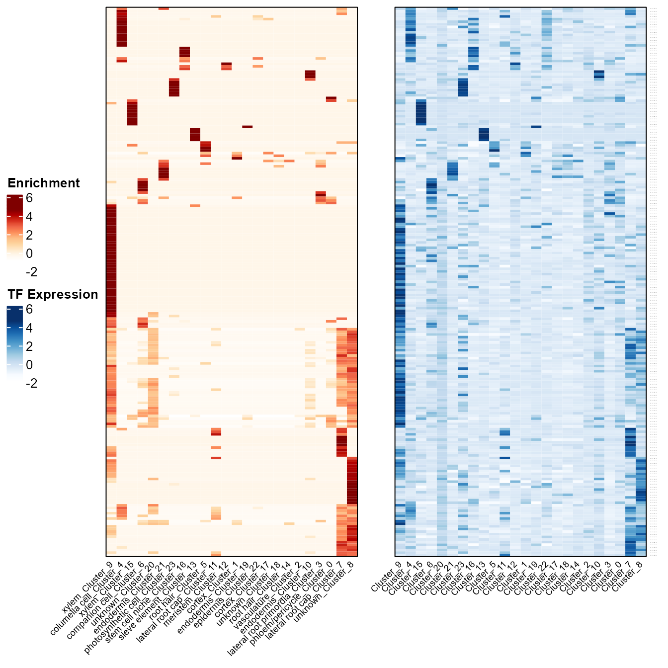
Dimension reduction plot showing cluster enrichment and TF expression.
enrich_exp_scatter(SeuratObj, MINIEXouputPath, gene = 'AT1G75390')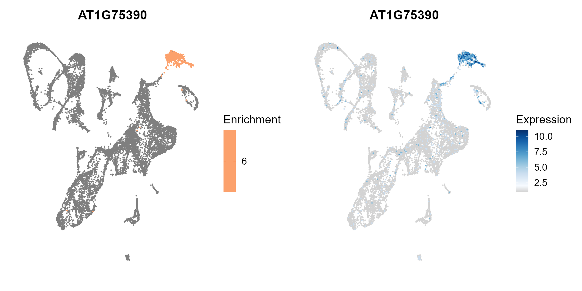
Network diagram showing top regulons of each cluster according to Borda ranking.
topRegulons_MINIEX(MINIEXouputPath, topn = 5)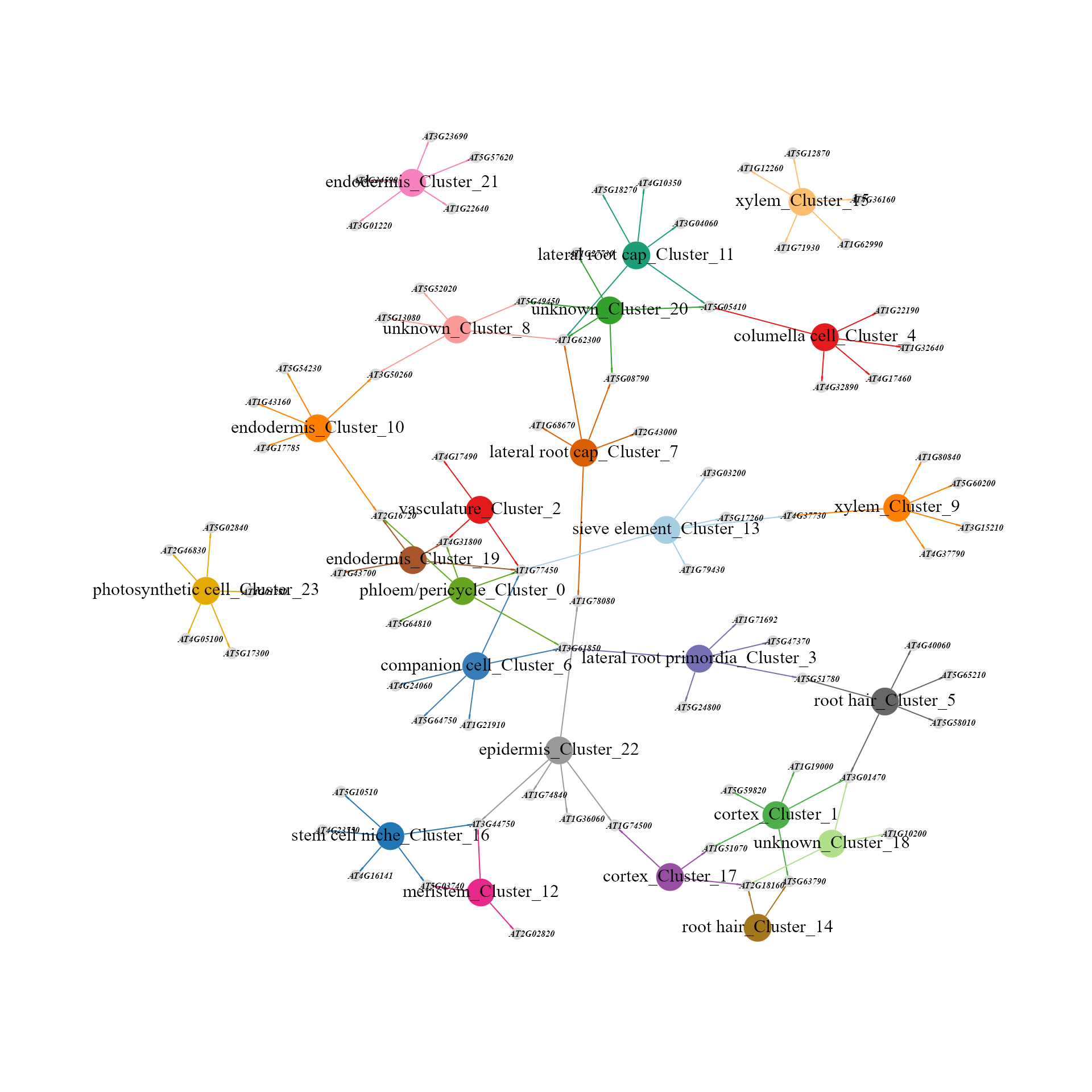
Network diagram showing targets of each regulon.
targets_MINIEX(MINIEXouputPath, cluster = 23, regulons = "AT3G16770")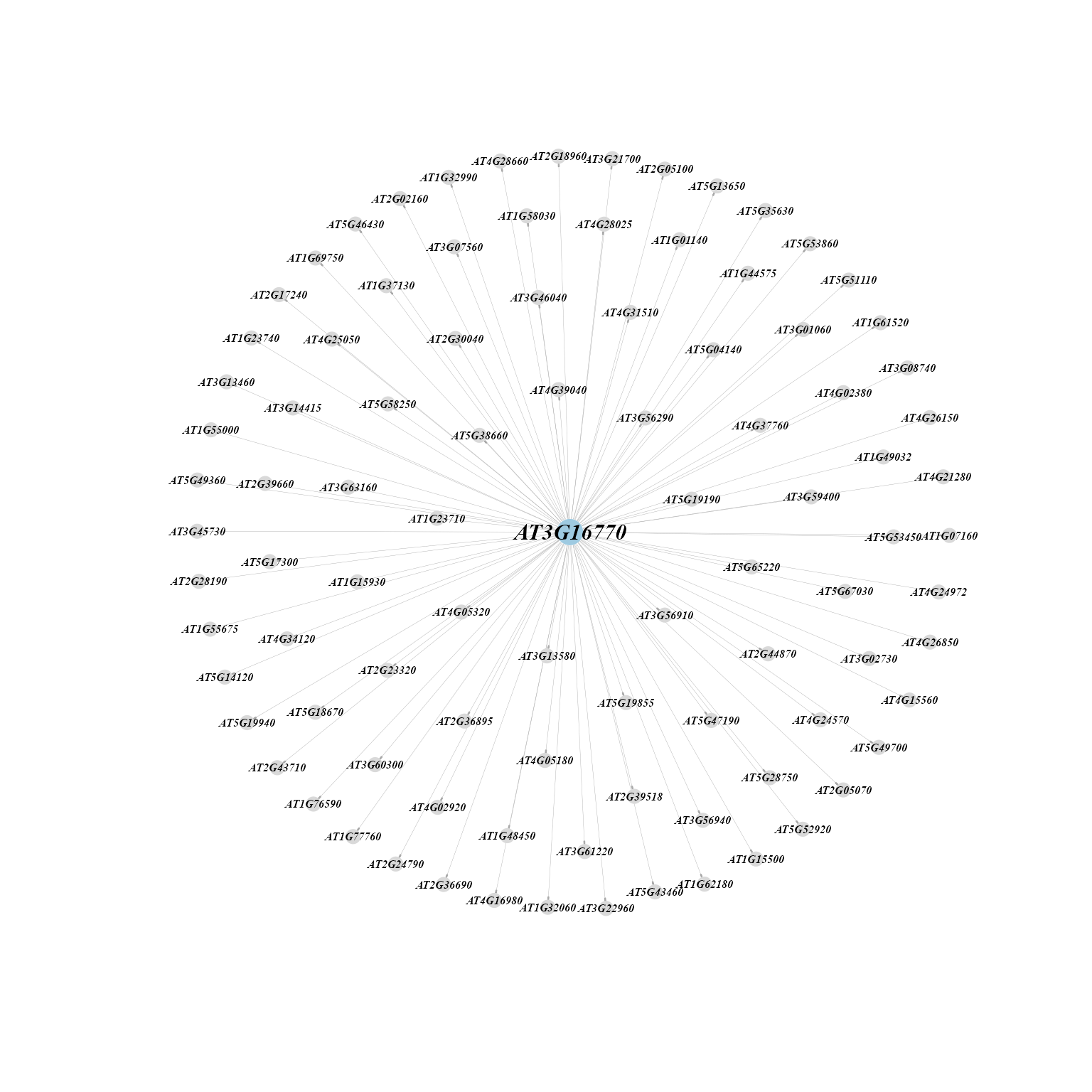
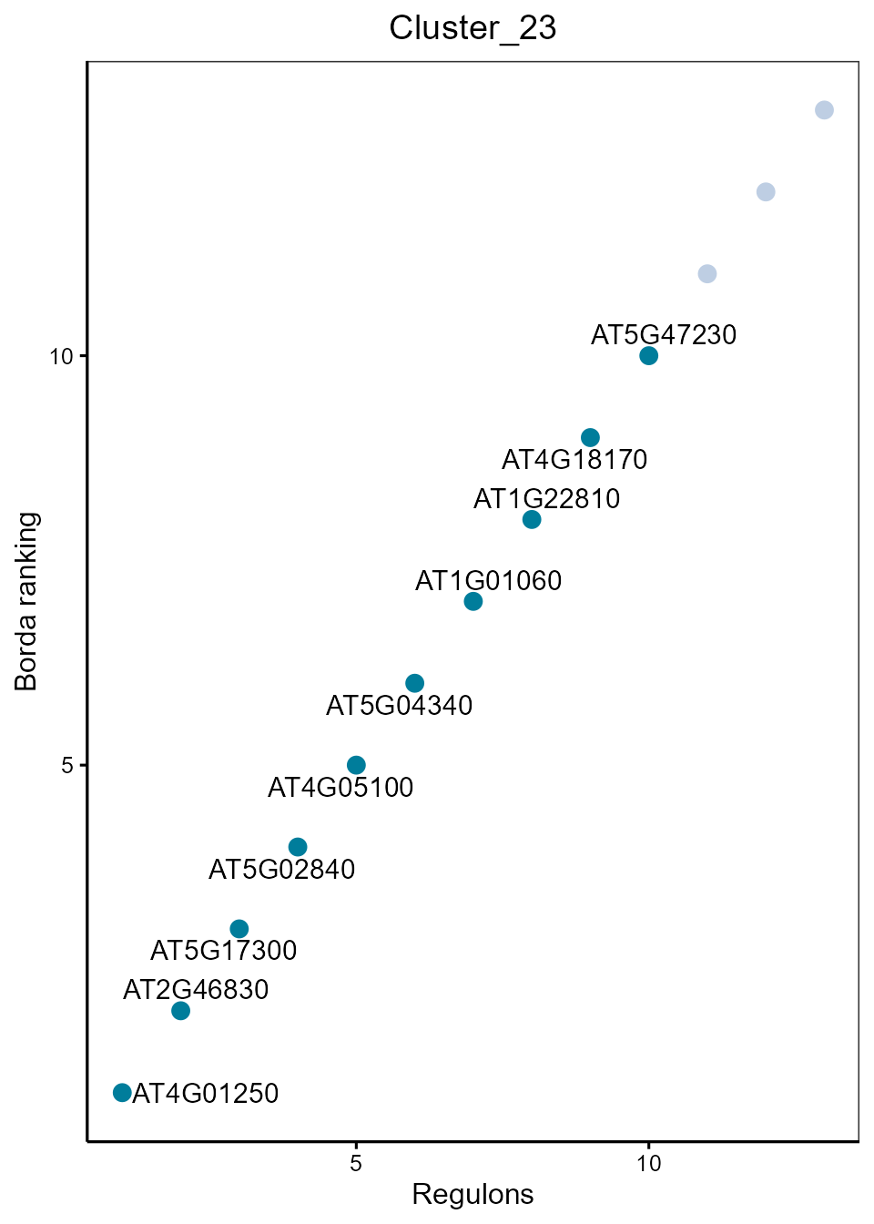
Dot plot showing top regulons of each cluster according to Borda ranking.
BordaRank_MINIEX(MINIEXouputPath, cluster=23, topn = 10)